Visualizing point distributions on a triangle mesh surface ↩

aliases: []
shorthands: {}
created: 2022-03-01 12:01:52
modified: 2022-07-11 13:29:30

Description of the method

For this, we take every single point in the point set and project them orthogonally to the closest triangles to determine that which triangles "own" which points. Then we can calculate a density for each triangle like this:

Where is the area of the triangle and is the number of points corresponding to it.

NOTE: If a single point corresponds to more than one triangle, we equally distribute it among the common triangles, so is not necessarily a whole number.

Algorithm

Now we show an implementation of this method in Python. We use numpy arrays and a method from scipy, so they have to be imported:

import numpy as np
from scipy.spatial import KDTree

First we implement a function for calculating the areas of the triangles:

def triangle_areas(x, y, z, i, j, k):
    v1x = x[j] - x[i]
    v2x = x[k] - x[i]
    v1y = y[j] - y[i]
    v2y = y[k] - y[i]
    v1z = z[j] - z[i]
    v2z = z[k] - z[i]

    crossx = v1y * v2z - v1z * v2y
    crossy = v1z * v2x - v1x * v2z
    crossz = v1x * v2y - v1y * v2x
    areas = 0.5 * np.sqrt(crossx**2 + crossy**2 + crossz**2)
    return areas

This returns a numpy with numbers corresponding to the areas of the triangles.

Then we implement the projector method in_triangle which determines if the given px, py, pz point projects to the triangle or not:

# Helper functions
def cross_prod(v1, v2):
    return (v1[1] * v2[2] - v1[2] * v2[1], v1[2] * v2[0] - v1[0] * v2[2], v1[0] * v2[1] - v1[1] * v2[0])


def dot_prod(v1, v2):
    return v1[0] * v2[0] + v1[1] * v2[1] + v1[2] * v2[2]


def in_triangle(x1, y1, z1, x2, y2, z2, x3, y3, z3, px, py, pz):
    v1 = (x2 - x1, y2 - y1, z2 - z1)
    v2 = (x3 - x2, y3 - y2, z3 - z2)
    v3 = (x1 - x3, y1 - y3, z1 - z3)
    normal = cross_prod(v1, v2)
    in1 = cross_prod(v1, normal)
    in2 = cross_prod(v2, normal)
    in3 = cross_prod(v3, normal)
    rel1 = ((-x1.T + px).T, (-y1.T + py).T, (-z1.T + pz).T)
    rel2 = ((-x2.T + px).T, (-y2.T + py).T, (-z2.T + pz).T)
    rel3 = ((-x3.T + px).T, (-y3.T + py).T, (-z3.T + pz).T)
    tr1 = (dot_prod(rel1, in1) <= 0)
    tr2 = (dot_prod(rel2, in2) <= 0)
    tr3 = (dot_prod(rel3, in3) <= 0)
    return np.logical_and(np.logical_and(np.equal(tr1, tr2), np.equal(tr1, tr3)), np.equal(tr2, tr3))

A function for smoothing the results is also built in for the sake of robustness:

def gauss_blur_point_set(x, y, z, values, sigma=1.0):
    result_values = []

    for i in range(len(x)):
        d = ((x[i] - x)**2 + (y[i] - y)**2 + (z[i] - z)**2)
        result_values.append(np.sum((np.e ** (-d / sigma)) * np.array(values)))

    return np.array(result_values)

This just applies a filter on the values in space according to the Gaussian function.

Now we can implement the function that evaluates the surface density:

def points_on_face(x, y, z, i, j, k, points_x, points_y, points_z, blur=False, blur_sigma=1.0):
    x = np.array(x)
    y = np.array(y)
    z = np.array(z)
    i = np.array(i)
    j = np.array(j)
    k = np.array(k)
    # Center of mass points
    com_x = (x[i] + x[j] + x[k]) / 3.0
    com_y = (y[i] + y[j] + y[k]) / 3.0
    com_z = (z[i] + z[j] + z[k]) / 3.0

    # Transform them to be able to use them in KDTree
    com_points = np.array([com_x, com_y, com_z]).T
    points = np.array([points_x, points_y, points_z]).T

    tree = KDTree(com_points)

    _, idx = tree.query(points, 7)
    point_indices = np.fromiter(range(len(idx)), dtype="int")
    is_eligible = in_triangle(x[i[idx]], y[i[idx]], z[i[idx]],
                                        x[j[idx]], y[j[idx]], z[j[idx]],
                                        x[k[idx]], y[k[idx]], z[k[idx]],
                                        points_x[point_indices], points_y[point_indices], points_z[point_indices])

    counts = np.zeros(len(i), dtype="float64")
    for idx_toadd in range(len(idx)):
        eligible_sum = np.sum(is_eligible[idx_toadd])
        if eligible_sum != 0:
            counts[idx[idx_toadd][is_eligible[idx_toadd]]
                   ] += (1.0 / eligible_sum)

    areas = triangle_areas(x, y, z, i, j, k)

    # Normalize with the triangle areas
    result = counts / areas

    # If we want to apply the filter, then apply it wiht sigma smoothing
    if blur:
        result = gauss_blur_point_set(com_x, com_y, com_z, result, blur_sigma)

    return result

We pass the mesh in the x, y, z, i, j, k arguments and the points from which the density is determined, are given in three arrays points_x, points_y, points_z. blur can be set to True to apply the filter.

Example

Let's say we generated a sphere from an icosahedron and we also have a function that generates random points isotropically on the surface of the sphere with a "bump" where we have a lot more points localized. This function looks like this:

import numpy.random as random

def generate_randoms_on_sphere_with_bump(seed=0, N = 1000, bump_N = 200, bump_phi = 0, bump_theta = np.pi/2., bump_size=0.1):
    random.seed(seed)
    points_z = (random.rand(N) - 0.5) * 2.0
    thetas = np.arccos(points_z)
    phis = random.rand(N) * (2 * np.pi)
    points_x = np.cos(phis) * np.sin(thetas)
    points_y = np.sin(phis) * np.sin(thetas)

    bump_phis = random.normal(bump_phi, bump_size, bump_N)
    bump_thetas = random.normal(bump_theta, bump_size, bump_N)

    bump_z = np.cos(bump_thetas)
    bump_y = np.sin(bump_phis) * np.sin(bump_thetas)
    bump_x = np.cos(bump_phis) * np.sin(bump_thetas)

Where the arguments mean the following:

• seed=0: the seed for random number generation
• N: number of points to generate isotropically
• bump_N: number of points in the bump
• bump_phi: the center angle of the bump (see Spherical coordinate system)
• bump_theta: the center angle of the bump
• bump_size: characterizes the size of the dump

Then we can apply all these together:

x, y, z, i, j, k = generate_sphere_fibonacci(1, 1500)
x, y, z, i, j, k = generate_icosahedron(1)
x, y, z, i, j, k = subdivide_triangles(x, y, z, i, j, k, 4)
for n in range(len(x)):
        R = np.sqrt(x[n]**2 + y[n]**2 + z[n]**2)
        x[n] = x[n]/R
        y[n] = y[n]/R
        z[n] = z[n]/R

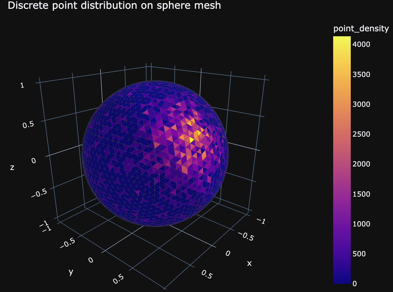
points_x, points_y, points_z = generate_randoms_on_sphere_with_bump(2324, 1000, 900, bump_phi=1.2, bump_theta=1.1, bump_size=0.3)

counts = points_on_face(x, y, z, i, j, k, points_x, points_y, points_z, blur=False, blur_sigma=0.01)

And if we visualize the calculated densities, we get the following figure:

Which was done with the following code snippet:

import plotly.graph_objects as go

# Create wireframe lines
Xe = []
Ye = []
Ze = []
for face_n in range(len(i)):
    Xe.append(x[i[face_n]])
    Xe.append(x[j[face_n]])
    Xe.append(x[k[face_n]])
    Ye.append(y[i[face_n]])
    Ye.append(y[j[face_n]])
    Ye.append(y[k[face_n]])
    Ze.append(z[i[face_n]])
    Ze.append(z[j[face_n]])
    Ze.append(z[k[face_n]])
    Xe.append(None)
    Ye.append(None)
    Ze.append(None)

fig = go.Figure(data=[
    go.Mesh3d(
        x=x, y=y, z=z,
        # i, j and k give the vertices of triangles
        i=i, j=j, k=k,
        name='y',
        showscale=True,
        colorbar_title='point_density',
        # Intensity of each fac
        intensity = counts,
        intensitymode='cell',
    ),
    go.Scatter3d(
        x=Xe,
        y=Ye,
        z=Ze,
        mode='lines',
        name='',
        line=dict(color= 'rgb(70,70,70)', width=1)
    ),
    go.Scatter3d(
        x=points_x,
        y=points_y,
        z=points_z,
        mode='markers',
        showlegend=False,
        visible=False,
        opacity=1,
    ),
])

fig.update_layout(title='Discrete point distribution on sphere mesh', margin={'autoexpand': True,'b': 5,'l': 5,'r': 5,'t': 30,}, autosize=True, width=700, height=500, template="plotly_dark")
fig.show()