Metadata
aliases: []
shorthands: {}
created: 2022-07-11 10:33:37
modified: 2022-07-11 11:06:08
Let's suppose that here, similar to the other methods, the shear zone is perpendicular to the
In this method we borrow some concepts from smoothed particle hydrodynamics to approximate the velocity at any given point in space for the granular material in question. We are going to use the particle approximation method, implemented in Python. Then, we can use the fact that in the kernel approximation of derivatives, the derivative of the quantity in question disappears, thus we only have to evaluate the derivative of the smoothing kernel function.
As a smoothing kernel, we chose simply the Gaussian function, which in Python is:
def gauss_kernel(r, h):
    return (h**3 / np.pi**(3/2)) * np.exp(-r**2 / h**2)
And we will be curious about the
def gauss_kernel_derivative_y(r, y, h):
    return -(2*h * y / np.pi**(3/2)) * np.exp(-r**2 / h**2)
Note that this function is not rotationally symmetric now, so we need to pass the y coordinate separately.
We also introduce a helper function to evaluate all of the particles' kernel functions in a given point in space:
def kernel_values(x, y, z, h):
    return gauss_kernel(np.sqrt((x-coords[:, 0])**2 + (y-coords[:, 1])**2 + (z-coords[:, 2])**2), h)
And using these as weights, we can evaluate the
def approximate_velocity(x, y, z, h):
    kernel_vals = kernel_values(x, y, z, h)
    return np.sum(kernel_vals * vs[:, 0]) / np.sum(kernel_vals)
Then we can do pretty much the same with the derivatives as well:
def kernel_derivative_y_values(x, y, z, h):
    return gauss_kernel_derivative_y(np.sqrt((x-coords[:, 0])**2 + (y-coords[:, 1])**2 + (z-coords[:, 2])**2), y-coords[:, 1], h)
def approximate_velocity_grad_y(x, y, z, h):
    kernel_vals = kernel_values(x, y, z, h)
    kernel_derivative_y_vals = kernel_derivative_y_values(x, y, z, h)
    return -np.sum(kernel_derivative_y_vals * vs[:, 0]) / np.sum(kernel_vals)
At first, just use these methods to approximate the velocities. We found that for the ellipsoidal particles, the h = 4*np.sqrt(a*b*c) smoothing factor was sufficient.
approximated_velocities = [approximate_velocity(
    co[0], co[1], co[2], 4*np.sqrt(a*b*c)) for co in coords]
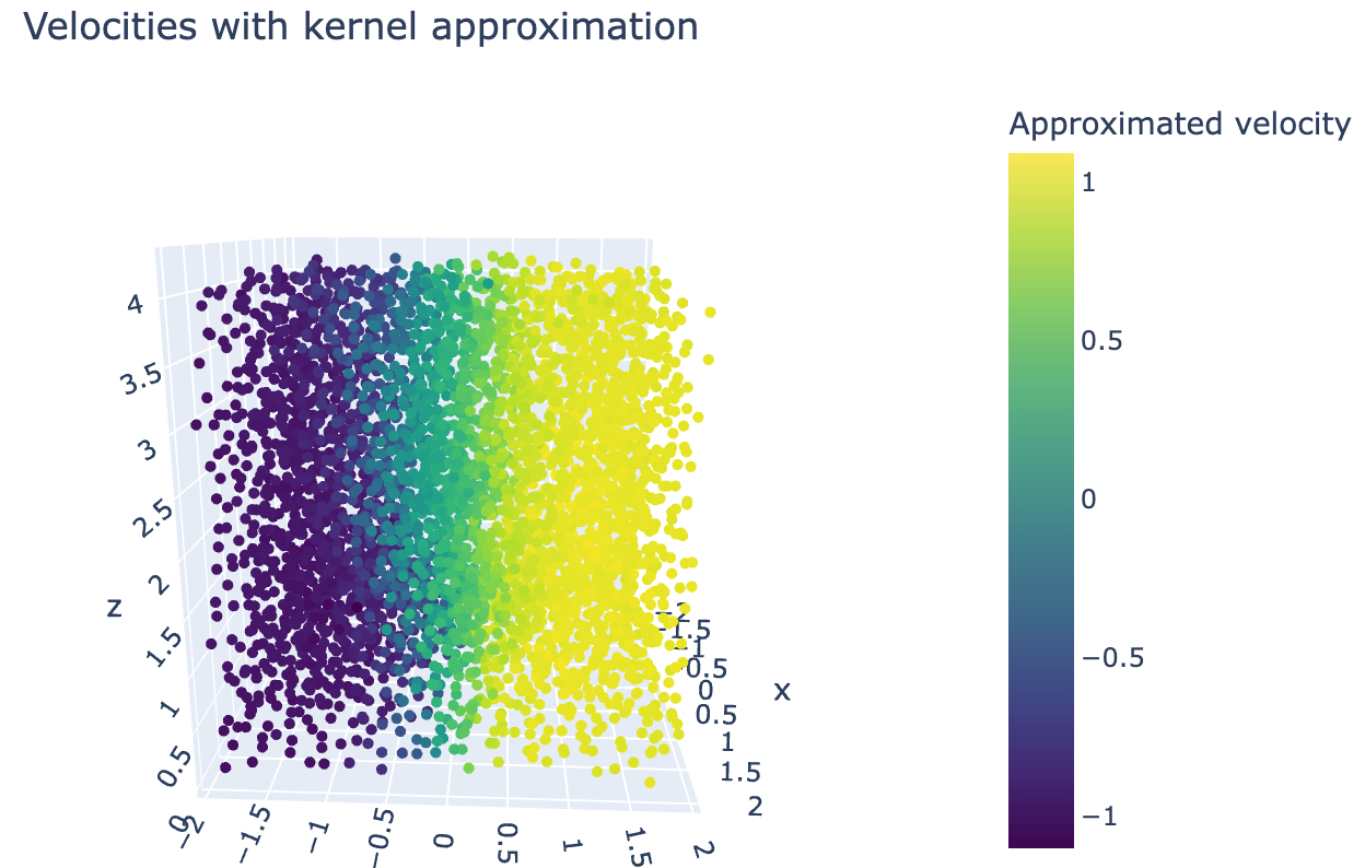
And we can plot the results:
fig = go.Figure(data=[go.Scatter3d(x=coords[:, 0], y=coords[:, 1], z=coords[:, 2],
                                   mode='markers',
                                   marker=dict(
    size=3, color=(approximated_velocities),
    colorscale='Viridis',
    colorbar=dict(title="Approximated velocity"),
    showscale=True))])
fig.update_layout(width=650, height=400, margin=dict(
    l=0, r=0, b=0, t=40), title="Velocities with kernel approximation")
fig.show()
We can see that this is very similar to the plot of the original data, just with a little bit of smoothing.
But what's more important is to be able to evaluate the gradient anywhere. This can be done similarly:
approximated_velocity_grads = [approximate_velocity_grad_y(
    co[0], co[1], co[2], 5*np.sqrt(a*b*c)) for co in coords]
And plotting it gives:
fig = go.Figure(data=[go.Scatter3d(x=coords[:, 0], y=coords[:, 1], z=coords[:, 2],
                                   mode='markers',
                                   marker=dict(
    size=3, color=(approximated_velocity_grads),
    colorscale='Viridis',
    colorbar=dict(title="Approximated shear rate"),
    showscale=True))])
fig.update_layout(width=650, height=400, margin=dict(
    l=0, r=0, b=0, t=40), title="Shear zone with kernel approximation")
fig.show()
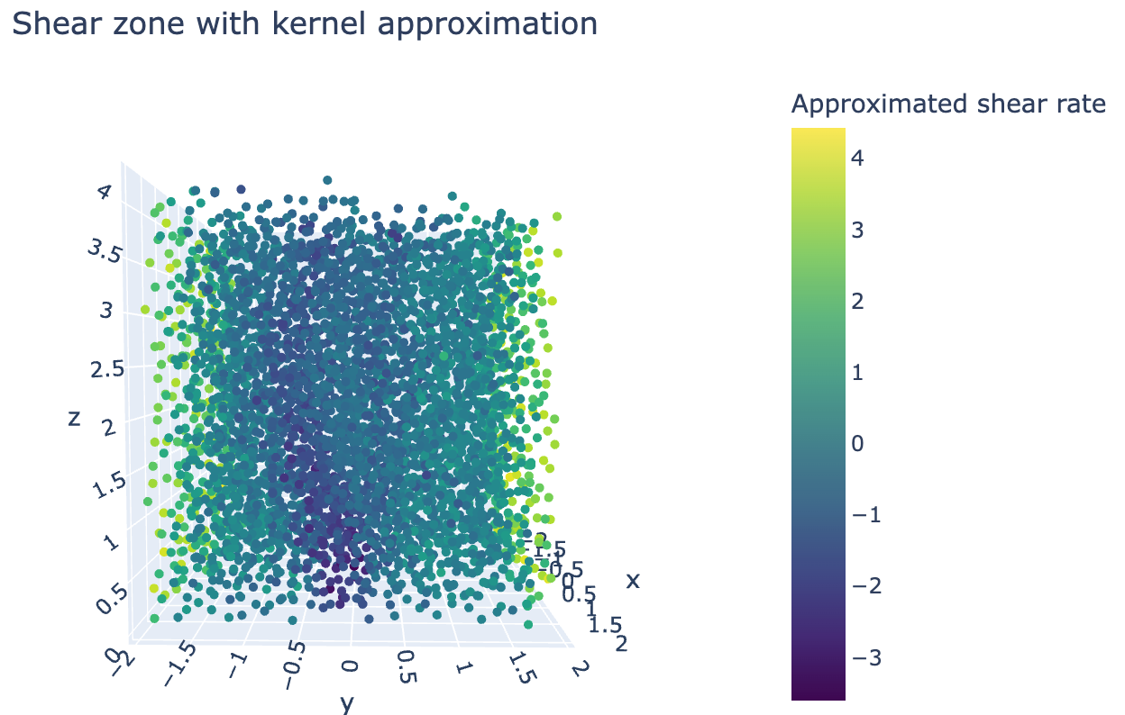
Which honestly does not look very promising. The reason for that is that we do not have boundary conditions in this approximation, so on the sides, the shear rate (gradient) becomes very large, offsetting the colorscale.
If we filter the shear zone out though, we see the following:
approximated_velocity_grads = np.array(approximated_velocity_grads)
zone_filter = approximated_velocity_grads < -1.3
Plotting it:
fig = go.Figure(data=[go.Scatter3d(x=coords[:, 0][zone_filter], y=coords[:, 1][zone_filter], z=coords[:, 2][zone_filter],
                                   mode='markers',
                                   marker=dict(
    size=3, color=(approximated_velocity_grads[zone_filter]),
    colorscale='Viridis',
    colorbar=dict(title="Approximated shear rate"),
    showscale=True))])
fig.update_layout(width=650, height=400, margin=dict(
    l=0, r=0, b=0, t=40), title="Shear zone with kernel approximation, everything else excluded", scene_aspectmode='cube')
fig.update_layout(
    scene=dict(
        xaxis=dict(range=[-2, 2],),
        yaxis=dict(range=[-2, 2],),
        zaxis=dict(range=[-0, 4],))
)
fig.show()
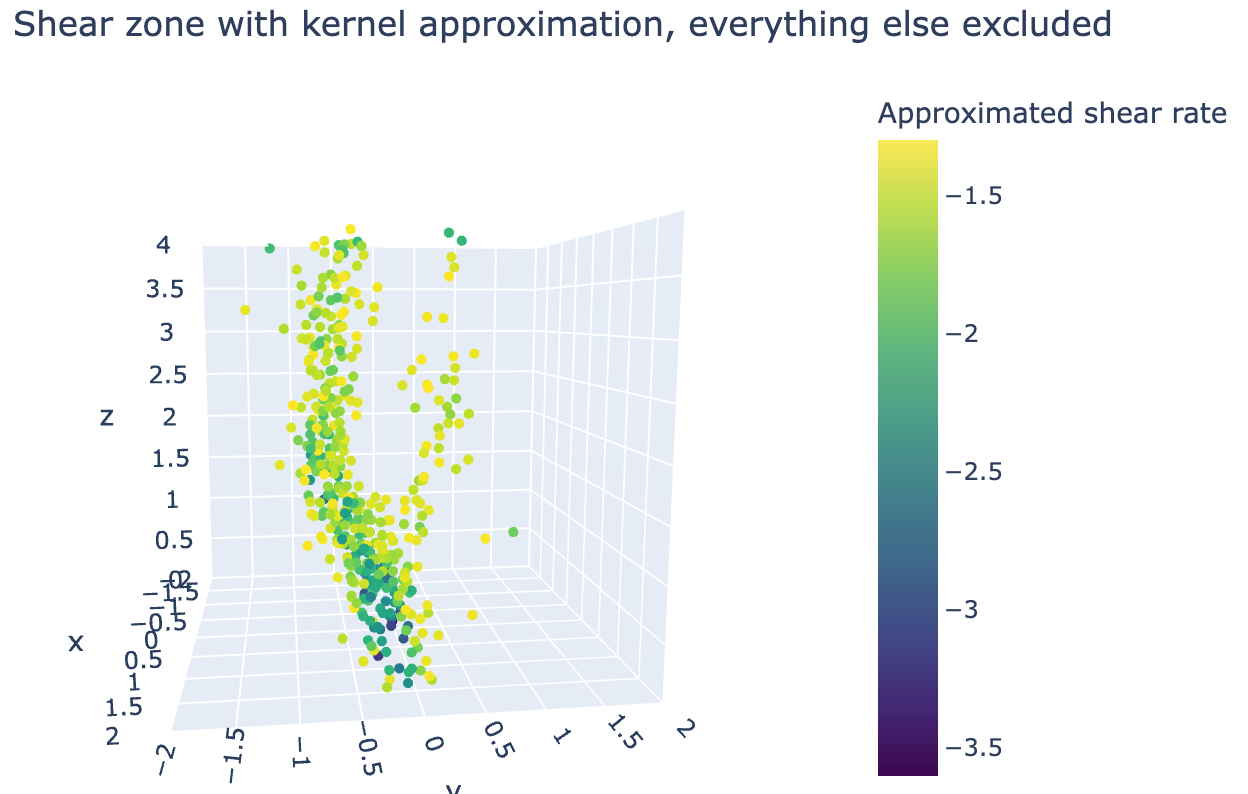
Which shows that this method gives a very detailed filtering method for the shear zone. It is also capable of detecting both branches of the shear zone, something that previous methods are not capable of doing.